Scaling Book Part 1. All About Rooflines

Roofline Model Fundamentals

When running algorithms on hardware, we’re bound by three fundamental constraints:

1. Compute Speed: How fast the hardware can do math operations (FLOPs/second)
2. Bandwidth: How quickly data can be moved around (bytes/second)
3. Memory Capacity: Total available storage for data (bytes)

These “Roofline” constraints help us establish upper and lower bounds for computation time.

Time Estimation Formulas

Computation Time

$T_{math}=\frac{\text{Computation FLOPs}}{\text{Accelerator FLOPs/s}}$

Example:

• H100 GPU: ~9.89e14 BFloat16 FLOPs/s
• TPU v6e: ~9.1e14 FLOPs/s

Communication Time

$T_{comms}=\frac{\text{Communication Bytes}}{\text{Network/Memory Bandwidth Bytes/s}}$

Communication happens in two main contexts:

• Within a chip: Transfers between on-chip memory (HBM) and compute cores
• Between chips: When distributing models across multiple accelerators

Time Bounds

• Lower bound: $T_{lower}=\max (T_{math},T_{comms})$
• Upper bound: $T_{upper}=T_{math}+T_{comms}$

In practice, we optimize toward the lower bound by overlapping communication and computation.

Arithmetic-Intensity

Definition: The ratio of total FLOPs performed to the number of bytes communicated.

$\text{Arithmetic Intensity} = \frac{\text{Computation FLOPs}}{\text{Communication Bytes}}$$

This measure (FLOPs/byte) determines whether an operation will be compute-bound or communication-bound:

• High intensity: Fully utilizes available FLOPs (compute-bound)
• Low intensity: Wastes FLOPs while waiting for data (communication-bound)

The crossover point is the “peak arithmetic intensity” of the hardware:

$\text{Peak Arithmetic Intensity}=\frac{\text{Peak Accelerator FLOPs/s}}{\text{Bandwidth Bytes/s}}$

For TPU v5e MXU, this is ~240 FLOPs/byte (1.97e14 FLOPs/s ÷ 8.2e11 bytes/s).

Example: Dot Product

For a dot product operation (x • y), where x and y are bfloat16 vectors of length N:

$\text{Intensity(dot product)}=\frac{N+N-1}{2N+2N+2}=\frac{2N-1}{4N+2}\approx \frac{1}{2}$

With an intensity of 0.5 FLOPs/byte, dot product operations are communication-bound on most hardware.

Visualizing Rooflines

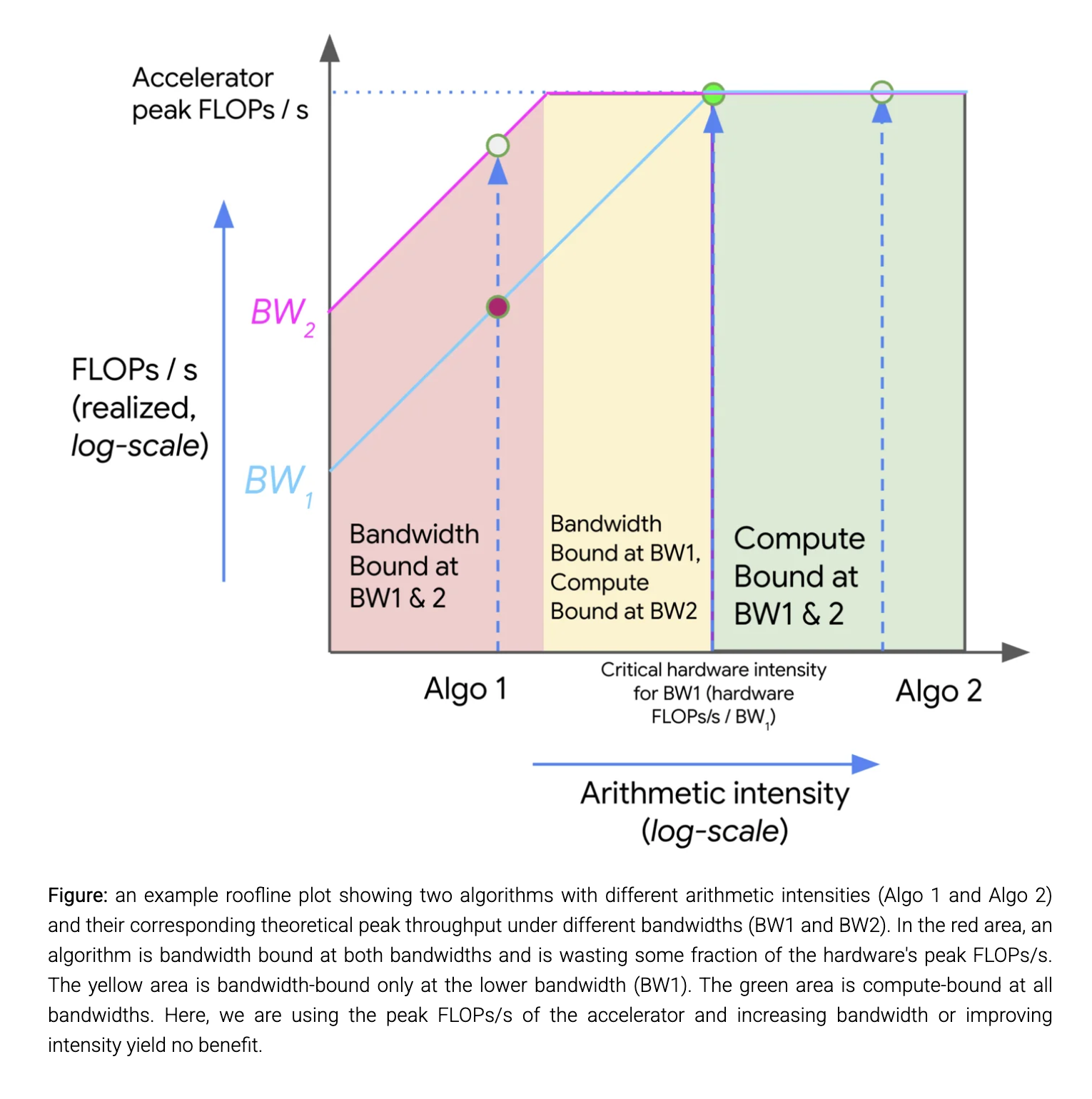Source: How To Scale Your Model - Rooflines

A roofline plot shows the relationship between arithmetic intensity (x-axis) and achievable performance in FLOPs/s (y-axis). The plot has three regions:

1. Red area: Bandwidth-bound at all bandwidths
2. Yellow area: Bandwidth-bound at lower bandwidths only
3. Green area: Compute-bound at all bandwidths

Performance can be improved by:

• Increasing arithmetic intensity of algorithms
• Increasing available memory bandwidth

Matrix-Multiplication Analysis

For matrix multiplication X * Y → Z where:

• X has shape bf16[B, D]
• Y has shape bf16[D, F]
• Z has shape bf16[B, F]

$\text{Intensity(matmul)}=\frac{2BDF}{2BD+2DF+2BF}=\frac{BDF}{BD+DF+BF}$

When the local batch size B is small relative to D and F (typical in Transformers):

$\text{Intensity(matmul)}\approx B$

Key Takeaway

For a bfloat16 matrix multiplication to be compute-bound on most TPUs, the local batch size in tokens needs to be greater than 240 (~300 for GPUs)

Network Communication Rooflines

When matrices are split across multiple accelerators, we need to consider inter-chip communication rooflines.

e.g. For a matrix multiplication split across 2 TPUs:

• Each TPU does half the work: $T_{math}=\frac{BDF}{1.97e14}$
• Communication time is: $T_{comms}=\frac{2BF}{4.5e10}$

The operation becomes compute-bound when: $\frac{D}{2}>\frac{1.97e14}{4.5e10}=4377$ or $Intensity(matmul(2-chips))>Intensity(Chipw.r.tinter-chipnetwork)$

Unlike the single-chip case, the critical threshold depends on D, not B. Why?

Cause D is now no longer factors in the data being moved, but B and F still do. Since B and F are both a factor in # FLOPs and data being moved, only B determines bottleneck.