Scaling Book Part 3. Sharded Matrices and How to Multiply Them

Sharding Matrices

When training large models across many TPUs, we need to split up arrays that don’t fit in the memory of a single accelerator. This process is called sharding or partitioning.

Partitioning Notation

A sharded array has two important shapes:

• Global/logical shape: The total shape of the unsharded array
• Device local shape: The actual size that each device holds

Device Mesh and Named-Axis Notation

We use a variant of named-axis notation to describe how tensors are sharded across devices:

1. Device Mesh: A 2D or 3D grid of devices with assigned mesh axis names (X, Y, Z)
2. Sharding: Assignment of tensor dimensions to mesh axes

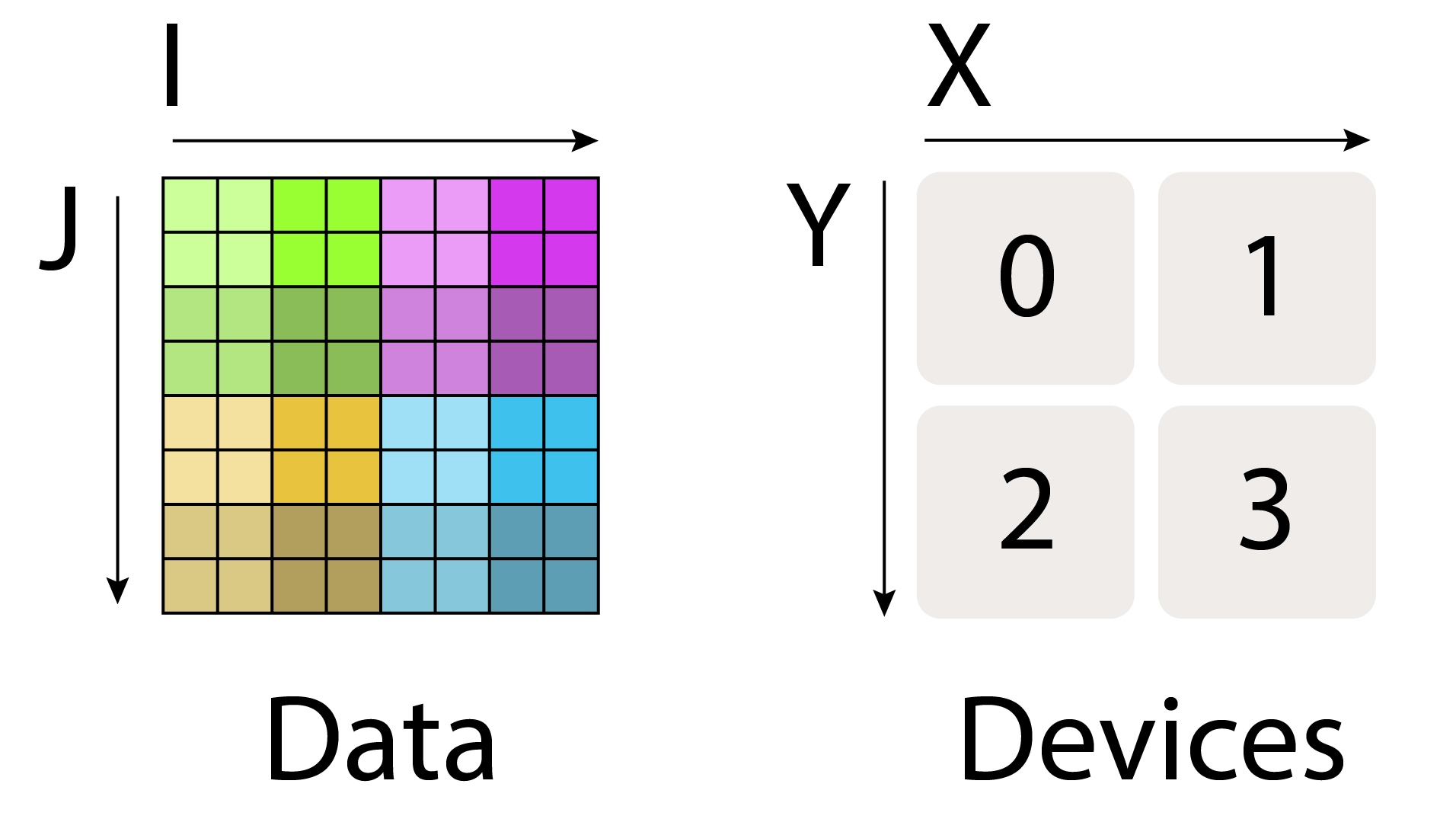Figure: Axes notations used for data and mesh (in this book). Source: How to Scale Your Model

Sharding Notation Examples

• A[I, J]: Fully replicated (each device has a complete copy)
• A[I_X, J]: First dimension sharded along X mesh axis, second dimension replicated
• A[I_X, J_Y]: First dimension sharded along X, second along Y
• A[I_XY, J]: First dimension sharded along both X and Y (flattened)

The local shape depends on the global shape and sharding pattern. For example, with A[I_X, J_Y], each device’s local shape is (|I|/|X|, |J|/|Y|).

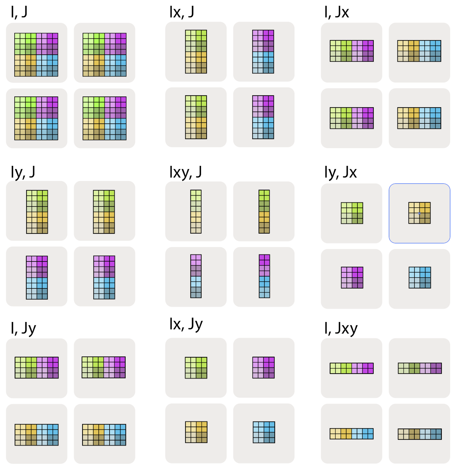Figure: Sharding configurations for a 2D matrix along a 2D mesh. Source: How to Scale Your Model

[! Important] We cannot have multiple dimensions sharded along the same mesh axis e.g., A[I_X, J_X] is invalid

JAX sharding example

import jax
import jax.numpy as jnp
import jax.sharding as shd
 
# Create our mesh! We're running on a TPU v2-8 4x2 slice with names 'X' and 'Y'.
assert len(jax.devices()) == 8
mesh = jax.make_mesh(axis_shapes=(4, 2), axis_names=('X', 'Y'))
 
# A little utility function to help define our sharding. A PartitionSpec is our
# sharding (a mapping from axes to names).
def P(*args):
  return shd.NamedSharding(mesh, shd.PartitionSpec(*args))
 
# We shard both A and B over the non-contracting dimension and A over the contracting dim.
A = jnp.zeros((8, 2048), dtype=jnp.bfloat16, device=P('X', 'Y'))
B = jnp.zeros((2048, 8192), dtype=jnp.bfloat16, device=P(None, 'Y'))
 
# We can perform a matmul on these sharded arrays! out_shardings tells us how we want
# the output to be sharded. JAX/XLA handles the rest of the sharding for us.
compiled = jax.jit(lambda A, B: jnp.einsum('BD,DF->BF', A, B), out_shardings=P('X', 'Y')).lower(A, B).compile()
y = compiled(A, B)

Computing with Sharded Arrays

Elementwise Operations

Elementwise operations on sharded arrays have no communication overhead – each device can operate independently on its local portion.

Matrix Multiplication with Sharded Arrays

Matrix multiplication between sharded arrays requires different communication patterns depending on how the arrays are sharded. There are four key cases:

Case 1: No Sharded Contracting Dimensions

When neither multiplicand has a sharded contracting dimension, we can multiply local shards without any communication:

$$A[I_X,J]\cdot B[J,K_Y]\to C[I_X,K_Y]$$

This works because the computation is independent of the sharding - each device has the complete data it needs for its portion of the output.

All of these cases follow this rule:

• $A[I,J]\cdot B[J,K]\to C[I,K]$
• $A[I_X,J]\cdot B[J,K]\to C[I_X,K]$
• $A[I,J]\cdot B[J,K_Y]\to C[I,K_Y]$
• $A[I_X,J]\cdot B[J,K_Y]\to C[I_X,K_Y]$

Case 2: One Sharded Contracting Dimension

When one multiplicand has a sharded contracting dimension, we typically perform an AllGather operation:

$$A[I,J_X]\cdot B[J,K]\to C[I,K]$$

First, gather all shards of A:

$${\text{AllGather}}_X(A[I,J_X])\to A[I,J]$$

Then multiply the fully gathered matrices:

$$A[I,J]\cdot B[J,K]\to C[I,K]$$

Case 3: Both Inputs Have Sharded Contracting Dimensions

When both inputs are sharded along the contracting dimension:

$$A[I,J_X]\cdot B[J_X,K]\to C[I,K]$$

We can:

1. Multiply local shards to get partial sums:

$$A[I,J_X]{\cdot }_{L}OCALB[J_X,K]\to C[I,K]U_X$$

2. Perform an AllReduce to sum the partial results:

$${\text{AllReduce}}_X(C[I,K]U_X)\to C[I,K]$$

Alternatively, we can use ReduceScatter followed by AllGather:

$$\begin{array}{r}A[I,J_X]{\cdot }_{LOCAL}B[J_X,K]\to C[I,K]U_X\\ {\text{ReduceScatter}}_X,K(C[I,K]U_X)\to C[I,K_X]\end{array}$$

Case 4: Invalid Sharding Pattern

When both multiplicands have a non-contracting dimension sharded along the same axis:

$$A[I_X,J]\cdot B[J,K_X]\to C[I_X,K_X]$$

This is invalid because each device would only compute a diagonal entry of the result.

To resolve this, we must AllGather one of the inputs first:

$$AllGathe{r}_X(A[I_X,J])\to A[I,J]A[I,J]\cdot B[J,K_X]\to C[I,K_X]$$

or:

$$AllGathe{r}_X(B[J,K_X])\to B[J,K]A[I_X,J]\cdot B[J,K]\to C[I_X,K]$$

Communication Primitives

Core Communication Operations

TPUs use four fundamental communication primitives for distributed computation:

1. AllGather: Removes a subscript from a sharding by collecting shards
   • Syntax: $[A_X,B]\to [A,B]$
2. ReduceScatter: Removes an “unreduced” suffix by summing shards over that axis
   • Syntax: $[A,B]U_X\to [A,B_X]$
3. AllReduce: Removes an “unreduced” suffix without introducing new sharding
   • Syntax: $[A_X,B]U_Y\to [A_X,B]$
   • Can be composed as ReduceScatter + AllGather
4. AllToAll: Switch shard from one axis to the other in the mesh
   • Syntax: $[A_X,B]\to [A,B_X]$

Figure: Visual representation of the four communication primitives

Source: How to Scale Your Model

Communication Cost Analysis

For bandwidth-bound operations, the cost of communications depends on:

• The size of the input arrays
• The bandwidth of the links
• The communication primitive being used

Operation	Description	Runtime
AllGather	Gathers shards of an array	bytes / (bidirectional bandwidth * num_axes)
ReduceScatter	Sums partial results and reshards	Same as AllGather
AllReduce	Sums partial results without resharding	2 * AllGather
AllToAll	Transposes sharding between dimensions	AllGather / 4 (on bidirectional ring)

The cost of these operations does not depend on the number of devices (in bandwidth-bound regime), but only on the data volume and available bandwidth.

ReduceScatter in Backpropagation

An important relationship: ReduceScatter is the gradient operation of AllGather:

• If the forward pass has: ${\text{AllGather}}_X(A[I_X])\to A[I]$
• Then backward pass has: ${\text{ReduceScatter}}_X(A^{\prime }[I]U_X)\to A^{\prime }[I_X]$

This relationship is critical for understanding communication patterns in backward passes during training.